Python Program to Implement Steady State Equations Assignment Solution

Instructions

Objective

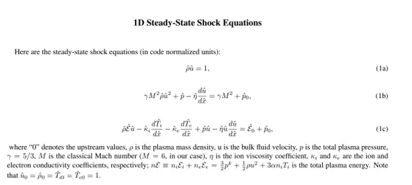
Write a python assignment program to implement steady state equations.

Requirements and Specifications

Source Code

import numpy as np import matplotlib.pyplot as plt M = 5.0 gam = 5./3. # ========================================================================== # ========================================================================== def ddx(x, F): Ns = F.size - 1 dFdx = np.zeros(Ns + 1, dtype='double') dFdx[0] = (F[1] - F[0]) / (x[1] - x[0]) for i in range(1, Ns): dFdx[i] = (F[i + 1] - F[i - 1]) / (x[i + 1] - x[i - 1]) dFdx[Ns] = (F[Ns] - F[Ns - 1]) / (x[Ns] - x[Ns - 1]) return dFdx # ========================================================================== # ========================================================================== if __name__ == '__main__': electron = np.loadtxt('./electron_quantites.txt') ion = np.loadtxt('./ion_quantites.txt') x = electron[:,0] # positions rho = ion[:,1] # this is rho/rho0. ke = electron[:,2] Te = electron[:,1] Ti = ion[:,2] ki = ion[:,3] eta = ion[:,4] u = ion[:,5] p = ion[:,6] E = ion[:,7] # First, calculate du/dx dudx = ddx(x, u) # Calculate dTi/dx dTidx = ddx(x, Ti) # Calculate dTe/dx dTedx = ddx(x, Te) # From equation (1b), calculate p0u0^2 + p0 eq1b = p + gam*M**2.*rho*u**2. - eta*dudx eq1b_right = gam*M**2 + p[0] # Equation (1c) eq1c = E*u + p*u - ki*dTidx - ke*dTedx - eta*u*dudx eq1c_right = E[0]/rho[0] + p[0] # Eq. 1a eq1a = rho*u #========================================================================== #========================================================================== # create plot plt.figure(figsize=(7,7)) # Plot dTidx plt.plot(x, rho, label = r'$\rho$') plt.plot(x, ke, label = '$k_{e}$') plt.plot(x, Te, label = '$T_{e}$') plt.plot(x, Ti, label = '$T_{i}$') plt.plot(x, ki, label = r'$k_{i}$') plt.plot(x, eta, label = r'$\eta$') plt.grid(True) plt.xlabel('Position') plt.legend() plt.show() plt.figure(figsize=(7,7)) plt.plot(x, u, label = 'u') plt.plot(x, p, label = 'p') plt.plot(x, E, label = 'E') plt.plot(x, dudx, label = r'$\frac{du}{dx}$') plt.plot(x, dTidx, label = r'$\frac{dT_{i}}{dx}$') plt.plot(x, dTedx, label = r'$\frac{dT_{e}}{dx}$') plt.xlabel('Position') plt.grid(True) plt.legend() plt.show() """ Now, plot each terms of each equation """ # Terms for Equation (1a) plt.figure() plt.plot(x, rho*u, label = r'$\rho u$') plt.xlabel('Position') plt.ylabel(r'$\rho u$') plt.set_title('Equation (1a)') plt.legend() plt.grid(True) plt.show() # Terms for question (1b). All terms in the same Figure # p + gam*M**2.*rho*u**2. - eta*dudx fig, axes = plt.subplots(nrows = 1, ncols = 2, figsize=(7,7)) axes[0].plot(x, p, label = r'$p$') axes[0].plot(x, gam*(M**2)*rho*(u**2), label = r'$\gamma M^{2}\rho u^{2}$') axes[0].plot(x, -eta*dudx, label = r'$-\eta \frac{du}{dx}$') axes[0].plot(x, eq1b, 'r--', label = r'$p + \gamma M^{2}\rho u^{2} - \eta \frac{du}{dx}$') axes[0].grid(True) axes[0].set_title('Left-side terms of Equation (1b)') axes[0].legend() axes[1].plot(x, gam*(M**2)*np.ones(len(x)), label = r'$\gamma M^{2}$') axes[1].plot(x, p[0]*np.ones(len(x)), label = r'$p_{0}$') axes[1].plot(x, eq1b_right*np.ones(len(x)), 'r--', label = r'$\gamma M^{2} + p_{0}$') axes[1].grid(True) axes[1].set_title('Right-side terms of Equation (1b)') axes[1].legend() plt.show() # Terms for Equation (1c). # E*u + p*u - ki*dTidx - ke*dTedx - eta*u*dudx = E[0]/rho[0] + p[0] fig, axes = plt.subplots(nrows = 1, ncols = 2, figsize=(7,7)) axes[0].plot(x, E*u, label = r'$Eu$') axes[0].plot(x, p*u, label = r'$pu$') axes[0].plot(x, -ki*dTidx, label = r'$-k_{i} \frac{dT_{i}}{dx}$') axes[0].plot(x, -ke*dTedx, label = r'$-k_{e} \frac{dT_{e}}{dx}$') axes[0].plot(x, -eta*u*dudx, label = r'$-\eta u \frac{du}{dx}$') axes[0].plot(x, eq1c, 'r--', label = r'$Eu + pu - k_{i} \frac{dT_{i}}{dx} - k_{e} \frac{dT_{e}}{dx} - \eta u \frac{du}{dx}$') axes[0].grid(True) axes[0].set_title('Left-side terms of Equation (1c)') axes[0].legend() axes[1].plot(x, E[0]/rho[0] *np.ones(len(x)), label = r'$\frac{E_{0}}{\rho_{0}}$') axes[1].plot(x, p[0]*np.ones(len(x)), label = r'$\rho_{0}$') axes[1].plot(x, eq1c_right*np.ones(len(x)), 'r--', label = r'$\frac{E_{0}}{\rho_{0}} + \rho_{0}$') axes[1].grid(True) axes[1].set_title('Right-side terms of Equation (1c)') axes[1].legend() plt.show() fig = plt.figure(figsize=(7, 5), dpi=120) plot = plt.plot(x, (eq1b-eq1b_right)/eq1b_right*100., 'royalblue', linestyle='--', label='Eq. (1b) percent error') plot = plt.plot(x, (eq1c-eq1c_right)/eq1c_right*100., 'tomato', linestyle='-', label='Eq. (1c) percent error') plot = plt.plot(x, (eq1a - 1.0)/1.0 *100, 'purple', linestyle='-', label = 'Eq. (1a) percent error') plt.ylabel(r'Percent error [%]') plt.xlabel(r'Position $\hat{x}$') #plt.xlim([25.0, 32.5]) plt.xlim([min(x), max(x)]) legend = plt.legend(loc='best', shadow=False, fontsize='small') #plt.savefig('equation_error.eps', format='eps', dpi=1000) plt.grid(True) plt.show() plt.close() #========================================================================== #==========================================================================