Create a Program to Implement Statistics Visualization in Python Assignment Solution

Instructions

Objective

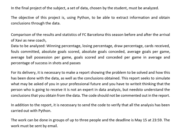
Write a python assignment program to implement statistics visualization.

Requirements and Specifications

Source Code

# Data visualization for Flights dataset ### Load needed library import pandas as pd import numpy as np import time import warnings warnings.filterwarnings('ignore') ### Import our Data df = pd.read_csv('flights.csv') # Data Overview df.head(100) df.shape ### know the number of columns and row of our dataset df.info() df.dtypes ### know the type of every column df.describe() ### Descriptive stats for our data df.isna().sum() ### Check if there is missing data df.duplicated().sum() ### we do not have any deuplicated rows df.nunique().to_frame().rename(columns={0:'Count'}) ### check the uniqueness of our columns row df['carrier'].unique() ### know how many carriers that we have in our dataset df['year'].unique() df.day.describe() print(df['carrier'].value_counts()) print(['WN: Southwest Airlines', 'AA: American Airlines', 'MQ: American Eagle Airlines', 'UA: United Airlines', 'OO: Skywest Airlines','DL: Delta Airlines','US: US Airways', 'EV: Atlantic Southeast Airlines','FL: AirTran Airways','YV: Mesa Airlines', 'B6: JetBlue Airways','9E: Pinnacle Airlines','AS: Alaska Airlines','F9: Frontier Airlines', 'HA: Hawaiian Airlines']) ### every airline and its frequency journies # Data cleaning ### see the missing data missing_data = df.isnull().sum(axis=0).reset_index() missing_data.columns = ['variable', 'missing values'] missing_data['filling factor (%)']=(df.shape[0]-missing_data['missing values'])/df.shape[0]*100 missing_data.sort_values('filling factor (%)').reset_index(drop = True) ### we see that those columns (air_time, arr_delay, arr_time, dep_time,dep_delay) have some missing data that we must handel df=df.dropna() ### remove any row with at least one missing value df.isna().sum() ### now no nulls cols=["day","month","year"] df['date'] = df[cols].apply(lambda x: '-'.join(x.values.astype(str)), axis="columns") ### join the coulmns day month year to one colmun to be the date of our data ### Setting the Frequency df.set_index("date", inplace=True) df.head() ### our data now sorted by the date # Exploratory Data Analysis import matplotlib.pyplot as plt import seaborn as sns import warnings warnings.filterwarnings('ignore') #correlation matrix corrmat = df.corr() f, ax = plt.subplots(figsize=(12, 9)) sns.heatmap(corrmat, vmax=.8, square=True); plt.show() ### this heatmap give us an intuation for the corrolation between our dataset columns which indicates that so coluns have very strong correlation like arrival time and departure time, other have so low correlation like arrival delay and distance. delay_type = lambda x:((0,1)[x > 5],2)[x > 45] fig = plt.figure(1, figsize=(10,7)) ax = sns.countplot(y="carrier", hue='year', data=df) # Setting Labels plt.setp(ax.get_xticklabels(), fontsize=12, weight = 'normal', rotation = 0); plt.setp(ax.get_yticklabels(), fontsize=12, weight = 'bold', rotation = 0); ax.yaxis.label.set_visible(False) plt.xlabel('Flight count', fontsize=16, weight = 'bold', labelpad=10) ### this count plot give us an observiation on which is the most airlines have made flights in 2013 ### we find that it is UA and B6 have most flights for 2014 where is very low flights for OO(SKYWEST) #Status on time (0), #slightly delayed (1), #highly delayed (2), for dataset in df: df.loc[df['arr_delay'] <= 10, 'Status'] = 0 df.loc[df['arr_delay'] >= 10, 'Status'] = 1 df.loc[df['arr_delay'] >= 30, 'Status'] = 2 f,ax=plt.subplots(1,2,figsize=(20,8)) df['Status'].value_counts().plot.pie(autopct='%1.1f%%',ax=ax[0],shadow=True) ax[0].set_title('Status') ax[0].set_ylabel('') sns.countplot('Status',order = df['Status'].value_counts().index, data=df,ax=ax[1]) ax[1].set_title('Status') plt.show() ### In 2013, a 71% of flights were delayed by more than 10 minutes. 12.9% of flights had delays of more than 10 min and less than half hour.On the other hand, 16.6% above hour delay = df[(df.Status >= 1) &(df.Status < 3)] #histogram sns.distplot(delay['arr_delay']) plt.show() ### It can be seen that delays are mostly located on the left side of the graph,The most of delays are short, and unusual we have very large delay fig = plt.figure(figsize=(20,8)) delay[['month','arr_delay']].groupby(['month']).mean().plot() plt.show() ### Delays focused on February, June and December, might the cause of the sumer and winter holidays fig = plt.figure(figsize=(20,8)) delay[['hour','arr_delay']].groupby(['hour']).mean().plot() plt.show() ### it is clear the the delays is rush between the 17:21 hour carrier_delay = df[['hour','carrier']].groupby(['carrier']).head() carrier_delay df.arr_delay.plot(figsize=(20,5)) plt.title("delays over 2013", size = 24) plt.ylim(0,1400) plt.show() f,ax=plt.subplots(1,figsize=(20,8)) sns.barplot('carrier','arr_delay', data=delay,ax=ax, order=['WN', 'AA','B6','AS', 'MQ', 'UA','OO','DL','US','EV','FL', 'YV', '9E','F9','HA'])

### We find the the Airlines 'OO: Skywest Airlines', 'YV: Mesa Airlines','9E: Pinnacle Airlines', and 'EV: Atlantic Southeast Airlines' have the most delays time along all the dataset. in other way the Airlines 'UA: United Airlines', 'AS: Alaska Airlines' have the least time delay over all carriers.