Matlab Program to Implement Range Equations Assignment Solution

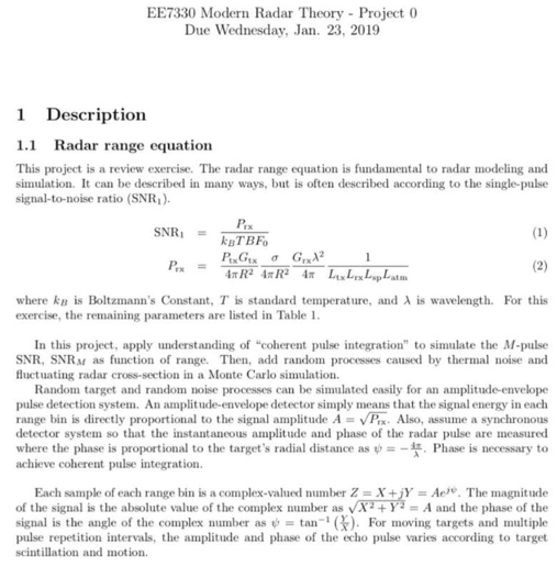
- Instructions
- Requirements and Specifications
Instructions
Requirements and Specifications


Source Code
% EE 7330 Modern Radar Theory
% Spring 2022 - Project 00
% Team 5
% Trevor Scarberry, Matthew Scharf, Siddhant Sharma
clc
clear all
close all
%% Parameters
%variables
Ptx = 150e3;
Fc = 9.4e9;
tau = 1.2e-6;
PRF = 2e3;
PRI = 1/PRF;
Gtx_dB = 45.25;
Tdw = 18.3e-3;
F0_dB = 2.5;
Ltx_dB = 3.1;
Lrx_dB = 2.4;
Lsp_dB = 3.2;
RT_km = 5:105;
RT = RT_km*1000;
Latm_dB = .16*2*RT_km;
sigma1_dB = 0;
sigma2_dB = -10;
SNRM_dB = 12;
% vT = [150 250 400] * 0.5144447;
vT = [150 250 400];
c = 3e8;
kB = 1.38e-23;
T = 290;
B = 1/tau;
lambda = c/Fc;
Rtgt_km = [25 50 70]; %target ranges, km
Rtgt = Rtgt_km * 1000;
Vtgt = [-15, 5, -10]; %Target velocities, m/s
%convert dB to abs
Gtx = 10^(Gtx_dB/10);
F0 = 10^(F0_dB/10);
Ltx = 10^(Ltx_dB/10);
Lrx = 10^(Lrx_dB/10);
Lsp =10^(Lsp_dB/10);
Latm = 10.^(Latm_dB/10);
SNRM = 10^(SNRM_dB/10);
sigma1 = 10^(sigma1_dB/10);
sigma2 = 10^(sigma2_dB/10);
np = floor(Tdw * PRF);
M = np;
L = Ltx*Lrx*Lsp.*(Latm);
N = kB*B*T*F0;
SNR_M_arr_dB = ones(1,length(RT)) * SNRM_dB; % Need array to plot
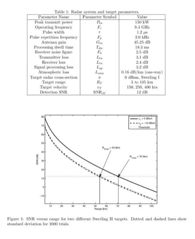
%% 1.a reproduce curves for SNRM versus range
Prx = (Ptx*Gtx^2*lambda^2)./((RT).^4*(4*pi)^3.*L); % here we calculate prc according to equation (2), but without the standard deviations
SNR0 = Prx./N;
% Here we complete the calculations of Prx and SNR for each standard
% deviation (positive and negative)
Prx1 = Prx*sigma1;
SNR1 = M*Prx1/(N);
Prx2 = Prx*sigma2;
SNR2 = M*Prx2/(N);
figure;
plot(RT_km, 10*log10(SNR1), '-b', 'LineWidth', 2);
hold on;
plot(RT_km, 10*log10(SNR2),'-k', 'LineWidth', 2);
hold on;
plot(RT_km, SNR_M_arr_dB,'r--', 'LineWidth', 2);
ylabel('SNR (dB)');
xlabel('Range (km)');
title('SNR vs Range')
legend('\sigma_1 = 0 dBsm ', '\sigma_2 = -10 dBsm','Threshold');
grid on;
xlim([min(RT_km) max(RT_km)]);
%% 1.b monte carlo sim
% we simulate 1000 events of randomness
for n = 1:1000
RCS1 = random('exp',sigma1,[M 1]);
RCS2 = random('exp',sigma2+1,[M 1]);
y1a(n,:) = sum(RCS1)*SNR1/M;
y2a(n,:) = sum(RCS2)*SNR2/M;
end
%obtain mean and standard deviation
y1avg = mean(y1a,1);
y1std = std(y1a,1,1);
y2avg = mean(y2a,1);
y2std = std(y2a,1,1);
%convert to db, create data for plots
y1avg_dB = 10*log10(y1avg);
y1avg_plus_std = 10*log10(y1avg+y1std);
y1avg_minus_std = 10*log10(y1avg-y1std);
y2avg_dB = 10*log10(y2avg);
y2avg_plus_std = 10*log10(y2avg+y2std);
y2avg_minus_std = 10*log10(y2avg-y2std);
%plot
figure;
hold on;
plot(RT_km,y1avg_dB)
plot(RT_km,y1avg_plus_std)
plot(RT_km,y1avg_minus_std)
plot(RT_km, SNR_M_arr_dB,'r--', 'LineWidth', 2);
plot(RT_km,y2avg_dB)
plot(RT_km,y2avg_plus_std)
plot(RT_km,y2avg_minus_std)
xlabel('Range[km]')
ylabel('SNR[dB]')
title('SNR vs Range (n=1000)')
legend('\sigma_1 = 0 dBsm ', '\sigma_2 = -10 dBsm','Threshold');
grid on;
xlim([min(RT_km) max(RT_km)]);
%% Part 2 - Range-Doppler Map
% here we calculate the signal amplitudes according toi equation (17.2) on
% the book
A = sqrt(Prx1);
% The next 3 lines calculates the amplitudes at each of the desired
% locations inside the range of study
A1= sqrt((Ptx*Gtx^2*sigma1*lambda^2)./((Rtgt(1))^4*(4*pi)^3.*L));
A2= sqrt((Ptx*Gtx^2*sigma1*lambda^2)./((Rtgt(2))^4*(4*pi)^3.*L));
A3= sqrt((Ptx*Gtx^2*sigma1*lambda^2)./((Rtgt(3))^4*(4*pi)^3.*L));
% The next line calculates the transmited frequency according to equation
% (17.1) on the book
Fd = 2*Vtgt/lambda;
%resolution = 1/(PRI*M);
% y1 = complex(zeros(length(RT_km),M));
% y2 = complex(zeros(length(RT_km),M));
% y3 = complex(zeros(length(RT_km),M));
%
% for l = 1:length(RT_km)
% for m = 1:M
%
% y1(l,m) = A(l)*exp(-1i*4*pi*Rtgt(1)/lambda)*exp(1i*2*pi*m*PRI*Fd(1));
% y2(l,m) = A(l)*exp(-1i*4*pi*Rtgt(2)/lambda)*exp(1i*2*pi*m*PRI*Fd(2));
% y3(l,m) = A(l)*exp(-1i*4*pi*Rtgt(3)/lambda)*exp(1i*2*pi*m*PRI*Fd(3));
% end
% end
% y0 = y1+y2+y3;
% Y =fftshift(fft(y0,[],2));
% Y1 = fftshift(fft(y1,[],2));
% Y2 = fftshift(fft(y2,[],2));
% Y3 = fftshift(fft(y3,[],2));
% We create the pulse-Doppler data matrix filled with zeros
y1 = complex(zeros(length(RT_km),M));
% Now, for every bin l0 and for every bin on the range M, we calculate
% the spatial Doppler signal
for l = 1:length(Rtgt_km)
for m = 1:M
idx = find(RT_km==Rtgt_km(l)); % One of the problems were here. The variable y1 has the same number
% of rows as elements in the vector
% RT_km, so when the values were
% changed for every value in
% Rtgt_km, the indices used were
% wrong
y1(idx,m) = A1(l)*exp(-1i*4*pi*Rtgt_km(l)/lambda)*exp(1i*2*pi*m*PRI*Fd(l));
end
end
% Now, we apply the fast fourier transform to the matrix and we obtain a
% complex number X + jY
Y1 = fftshift(fft(y1, [], 2), 2); % Another fix was done here. The fftshift and fft
% functions were called with
% incorrect arguments for number of
% dimensions
% Y2 = fftshift(fft(y2,[],2));
% Y3 = fftshift(fft(y3,[],2));
% Here we define the range of frequencies (x) and the space (y)
x = linspace((-PRF/2),(PRF/2),M);
y = linspace(min(RT_km),max(RT_km),length(RT_km));
%
% %plots
% figure
% hold on
% subplot(1,3,1)
% pcolor(x,y,abs((Y1)))
% title('range-doppler plot v = 150')
% xlabel('Doppler Freq (Hz)')
% ylabel('range(km)')
% shading interp
% colormap jet
% colorbar;
% subplot(1,3,2)
% pcolor(x,y,abs((Y2)))
% title('range-doppler plot v = 250')
% xlabel('Doppler Freq (Hz)')
% ylabel('range(km)')
% shading interp
% colormap jet
% colorbar;
% subplot(1,3,3)
% pcolor(x,y,abs((Y3)))
% title('range-doppler plot v = 400')
% xlabel('Doppler Freq (Hz)')
% ylabel('range(km)')
% shading interp
% colormap jet
% colorbar;
figure
hold on
pcolor(x,y,abs(Y1))
title('range-doppler plot')
xlabel('Doppler Freq (Hz)')
ylabel('range(km)')
xlim([-PRF/2,PRF/2]);
ylim([min(RT_km), max(RT_km)]);
shading interp
colormap jet
colorbar;
% figure;
% subplot(3,1,1)
% plot(x,abs(Y1))
% xlabel("Doppler Freq (Hz)");
% ylabel("Range (km)");
% % xlim([min(RT_km), max(RT_km)]);
% grid on;
% subplot(3,1,2)
% plot(x,abs(Y2))
% xlabel("Doppler Freq (Hz)");
% ylabel("Range (km)");
% % xlim([min(RT_km), max(RT_km)]);
% grid on;
% subplot(3,1,3)
% plot(x,abs(Y3))
% xlabel("Doppler Freq (Hz)");
% ylabel("Range (km)");
% % xlim([min(RT_km), max(RT_km)]);
% grid on;
Related Samples
Welcome to our Programming Assignments sample section, where learning meets excellence. Explore diverse programming challenges solved comprehensively for students. From introductory tasks to intricate projects, each example offers clear, step-by-step solutions. Enhance your programming skills with practical code examples covering various languages and concepts, tailored to enrich your learning experience.
Programming
Programming
Programming
Programming
Programming
Programming
Programming
Programming
Programming
Programming
Programming
Programming
Programming
Programming
Programming
Programming
Programming
Programming
Programming
Programming