Program To Implement Graph Plotting Assignment Solution.

Instructions

Objective

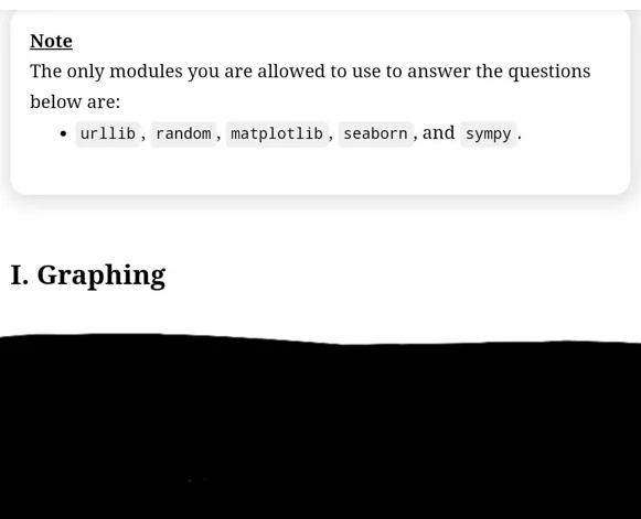
Write a Python assignment that involves creating a program to implement graph plotting in Python. Graph plotting is a fundamental skill in data visualization and analysis. Python offers various libraries like Matplotlib, Seaborn, and Plotly that enable users to create different types of graphs, such as line plots, bar plots, scatter plots, and more. These libraries provide functions to customize the appearance of graphs, add labels and titles, and handle data efficiently. By completing this assignment, students will gain practical experience in using Python libraries to visualize data and convey meaningful insights through graphical representations.

Requirements and Specifications

Source Code

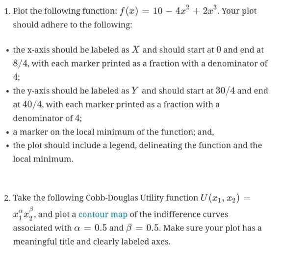
import matplotlib.pyplot as plt import seaborn as sns from sympy import * import urllib.request import random from sympy.plotting.plot import Plot, ContourSeries import numpy as np def Problem1(): print("Running problem 1...") # Create the symbolic variable x x = Symbol('x') # Create function f = 10 - 4 * x ** 2 + 2 * x ** 3 # Get its minimum fprime = f.diff(x) x_min = solve(fprime, x)[1] f_xmin = f.subs(x, x_min) # Plot #plot(f, (x, 0, 8 / 4), xlim=(0, 8 / 4), ylim=(30 / 4, 40 / 4), xlabel='X', ylabel='Y', label='Function', show = False) xvals = np.linspace(0, 8/4, 100) fvals = lambdify(x, f)(xvals) plt.figure() plt.plot(xvals, fvals, label = f) plt.plot(x_min, f_xmin,'r*', label = 'Local Minimum') plt.xlim([0, 8/4]) plt.ylim([30/4, 40/4]) plt.xlabel('X') plt.ylabel('Y') plt.legend() plt.xticks([0, 1/4, 2/4, 3/4, 4/4, 5/4, 6/4, 7/4, 8/4], ['0', '1/4', '2/4', '3/4', '4/4', '5/4', '6/4', '7/4', '8/4']) plt.yticks([30/4, 32/4, 34/4, 36/4, 38/4, 40/4], ['30/4', '32/4', '34/4', '36/4', '38/4', '40/4']) plt.show() """plt.xticks(['0', '1/4', '2/4', '3/4', '4/4', '5/4', '6/4', '7/4', '8/4']) plt.yticks([30/4, 31/4, 32/4, 33/4, 34/4, 35/4, 36/4, 37/4, 38/4, 39/4, 40/4]) plt.label() plt.show()""" def Problem2(): print("Running Problem 2...") # Define alpha and beta alpha = 0.5 beta = 0.5 # Define x1 and x2 x1 = Symbol("x1") x2 = Symbol("x2") graph = Plot(ContourSeries(x1**alpha *x2**beta, (x1, -100,100), (x2,-100,100)), xlabel = 'x1', ylabel = 'x2') graph.show() 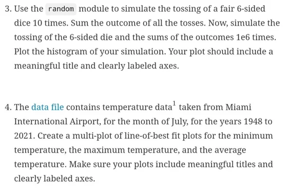def Problem3(): print("Running Problem 3...") # Now 1e6 times sum2 = [] for i in range(1000000): sum1 = 0 for i in range(10): die = random.randint(1, 6) sum1 += die sum2.append(sum1) # Now, plot histogram plt.figure() plt.hist(sum2) plt.xlabel('Sum of the outcomes') plt.ylabel('Number of times these sums were obtained') plt.show() def Problem4(): print("Running problem 4...") # Read file from link data= urllib.request.urlopen("https://raw.githubusercontent.com/AlR0d/courses/main/4465/miami_july_temps.csv").readlines() # process data # We delete the first entry in data because that line contains the header data.pop(0) # Create a list to store min_temp, max_temp and mean_temp min_temps = [] max_temps = [] mean_temps = [] # Now, process each line for line in data: line = line.decode('utf-8') line = line.rstrip() # Split using comma row = line.split(",") # Get min, max and mean temps min_temp = float(row[3]) max_temp = float(row[4]) mean_temp = float(row[5]) # Append min_temps.append(min_temp) max_temps.append(max_temp) mean_temps.append(max_temp) # Fit curve using seaborn # Now plot fig, axes = plt.subplots(nrows = 3, ncols = 1, figsize=(8,8)) x = np.linspace(0, len(min_temps)-1, len(min_temps)) sns.regplot(x=x, y=min_temps, ax = axes[0]) sns.regplot(x, max_temps, ax=axes[1]) sns.regplot(x, mean_temps, ax=axes[2]) axes[0].set_title('Min. 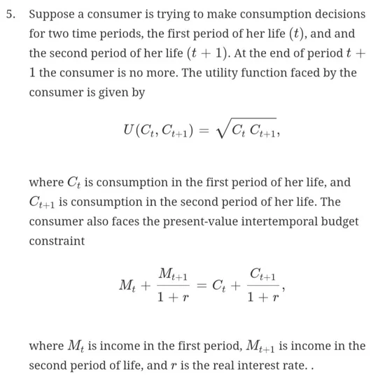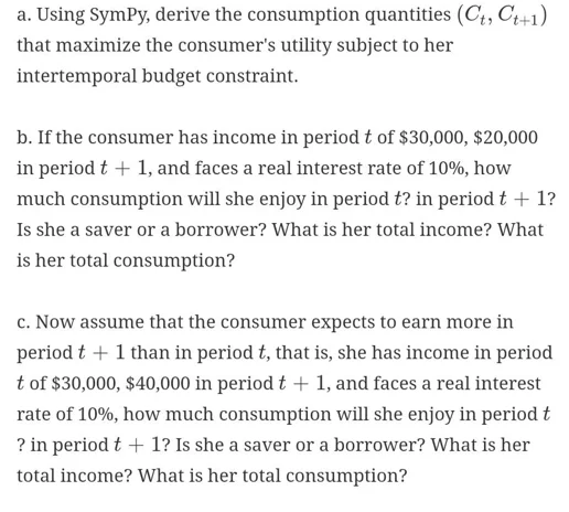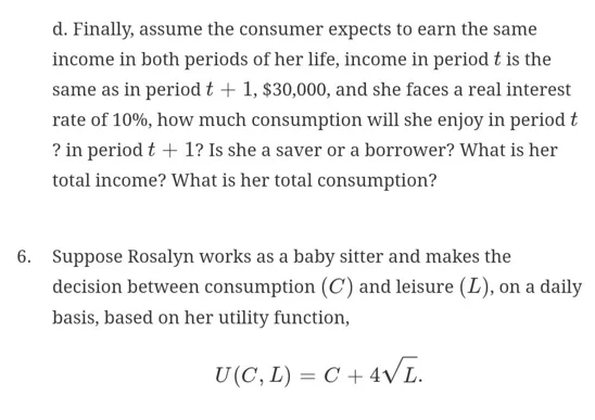Temp') axes[0].set_xlabel('Years since July 1948') axes[0].set_ylabel('Temperature') axes[1].set_title('Max Temp') axes[1].set_xlabel('Years since July 1948') axes[1].set_ylabel('Temperature') axes[2].set_title('Mean Temp') axes[2].set_xlabel('Years since July 1948') axes[2].set_ylabel('Temperature') plt.show() def Problem5(): print("Running problem 5...") """ part a """ # Define the variables Ct, Ct1, S = var('ct,ct1,s',real=True) # Define lambdas lam1 = symbols('lambda1',real = True) lam2 = symbols('lambda2', real=True) # Define r r = 0.1 # Define the objective function. NOTE: We set the objctive as negative in order to maixmize f = (Ct*Ct1)**(1/2) """ PART B """ print(" *** PART B *** ") # Define intertemporal budget constraint Mt = 30000 Mt1 = 20000 const1 = Mt - Mt1 / (1 + r) - Ct - Ct1 / (1 + r) # Define saving function const2 = S - Mt + Ct # Define lagrangian L = f - lam1 * const1 - lam2 * const2 # Define gradient gradL = [diff(L, c) for c in [Ct, Ct1, S]] KKT_eqs = gradL + [const1] + [const2] sol = solve(KKT_eqs, [Ct,Ct1,S,lam1,lam2],dict=True)[0] Ctsol = sol[Ct] Ct1sol = sol[Ct1] Ssol = sol[S] print("The consumption at period t is {:.2f}".format(Ctsol)) print("The consumption at period t+1 is {:.2f}".format(Ct1sol)) print("The savings are {:.2f}".format(Ssol)) print("The total income is {:.2f}".format(Mt+Mt1)) print("The toal consumption is {:.2f}".format(Ctsol+Ct1sol)) print() """ PART C """ print(" *** PART C *** ") # Define interporal budget constraint Mt = 30000 Mt1 = 40000 const1 = Mt - Mt1 / (1 + r) - Ct - Ct1 / (1 + r) # Define saving function const2 = S - Mt + Ct # Define lagrangian L = f - lam1 * const1 - lam2 * const2 # Define gradient gradL = [diff(L, c) for c in [Ct, Ct1, S]] KKT_eqs = gradL + [const1] + [const2] sol = solve(KKT_eqs, [Ct, Ct1, S, lam1, lam2], dict=True)[0] ctsol = sol[Ct] Ct1sol = sol[Ct1] Ssol = sol[S] print("The consumption at period t is {:.2f}".format(Ctsol)) print("The consumption at period t+1 is {:.2f}".format(Ct1sol)) print("The savings are {:.2f}".format(Ssol)) print("The total income is {:.2f}".format(Mt + Mt1)) print("The toal consumption is {:.2f}".format(Ctsol + Ct1sol)) print() """ PART D """ print(" *** PART D *** ") # Define interporal budget constraint Mt = 30000 Mt1 = 30000 const1 = Mt - Mt1 / (1 + r) - Ct - Ct1 / (1 + r) # Define saving function const2 = S - Mt + Ct # Define lagrangian L = f - lam1 * const1 - lam2 * const2 # Define gradient gradL = [diff(L, c) for c in [Ct, Ct1, S]] KKT_eqs = gradL + [const1] + [const2] sol = solve(KKT_eqs, [Ct, Ct1, S, lam1, lam2], dict=True)[0] Ctsol = sol[Ct] ; Ct1sol = sol[Ct1] Ssol = sol[S] print("The consumption at period t is {:.2f}".format(Ctsol)) print("The consumption at period t+1 is {:.2f}".format(Ct1sol)) print("The savings are {:.2f}".format(Ssol)) print("The total income is {:.2f}".format(Mt + Mt1)) print("The toal consumption is {:.2f}".format(Ctsol + Ct1sol)) print() 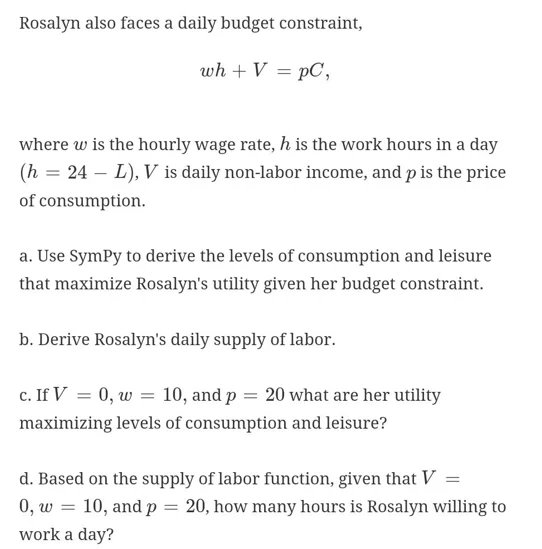def Problem6(): print("Running problem 6...") # Define parameters w = 10 V = 0 p = 20 # Define variables C, L = var('C,L', real=True) # Define lambda lam = symbols('lambda', real=True) # Define objective f = (C + 4*L**(1/2)) # Negative so we maximize it # Define the budget constraint constraint1 = w*(24 - L) + V - p*C # Define lagrangian Lag = f - lam * constraint1 # Define gradient gradL = [diff(Lag, c) for c in [C, L]] KKT_eqs = gradL + [constraint1] sol = solve(KKT_eqs, [C, L, lam], dict=True)[0] #print(sol) Csol = sol[C] Lsol = sol[L] fval = f.subs(C, Csol) fval = fval.subs(L, Lsol) """ Part b """ print("The consumption is {:.2f} and the leisure is {:.2f}".format(Csol, Lsol)) """ Part c """ print("The utility is {:.2f}".format(fval)) """ Part d """ print("Rosalyn is willing to work {:.0f} hours a day".format(24 - Lsol)) """ Part e """ # For this case, V = 14600/365 V = 14600/365 # We compute all variables again constraint1 = w * (24 - L) + V - p * C p; # Define lagrangian Lag = f - lam * constraint1 # Define gradient gradL = [diff(Lag, c) for c in [C, L]] KKT_eqs = gradL + [constraint1] sol = solve(KKT_eqs, [C, L, lam], dict=True)[0] #print(sol) Csol = sol[C] Lsol = sol[L] fval = f.subs(C, Csol) fval = fval.subs(L, Lsol) print("With the new law, Rosalyn is willing to work {:.0f} hours a day and her utility is {:.2f}".format(24 - Lsol, fval)) if __name__ == '__main__': Problem1() Problem2() Problem3() Problem4() Problem5() Problem6()