Create a Program to Implement Gradient Descent in Python Assignment Solution

Instructions

Objective

Write a python assignment program to implement gradient descent.

Requirements and Specifications

Source Code

In this quiz, you will: TODO #1. Debug my gradient descent implementation (5PTS for `dj_dw` and 5PTS for `dj_db`) to find the best parameters ($w$ and $b$) for the linear regression model being used. TODO #2. Play with the learning rate (5PTS for finding a good `alpha`). TODO # 3. Experiment with the learning rate value (5PTS to find the learning rate `alpha` that breaks the process). Note. - We're only covering the single feature case (only focused on the size of a house). - We're not concerned with testing. 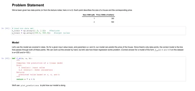import math, copy import numpy as np import matplotlib.pyplot as plt # Problem Statement We've been given two data points ($m$ from the lecture notes; here $m$ is 2). Each point describes the size of a house and the corresponding price. | Size (1000 sqft) | Price (1000s of dollars) | | ----------------| ------------------------ | | 1 | 300 | | 2 | 500 | # Load our data set x_train = np.array([1.0, 2.0]) #features y_train = np.array([300.0, 500.0]) #target values ### Model Let's use the model we covered in class. So for a given input value (size), and paramters ($w$ and $b$), our model can predict the price of the house. Since there's only data points, the correct model is the line that passes through both of these points. We can work out the answer by hand, but let's see how linear regression works problem. (Correct answer for a model of the form $f_{wb}(x) = wx + b$ on this dataset is w=200 and b=100.) def f_wb(x, w, b): """ Computes the prediction of a linear model Args: x (scalar): input value w,b (scalar): model parameters Returns predicted value based on x, w, and b """ return w * x + b We'll use `plot_predictions` to plot how our model is doing. def plot_predictions(x, y, w, b): """ Plots prediction model and actual values Args: x (ndarray(m,)): input values, m examples y (ndarray(m,)): output values, m examples (the correct answers) w,b (scalar): model parameters """ m = x.shape[0] predictions = np.zeros(m) for i in range(m): predictions[i] = f_wb(x[i], w, b) # Plot our model prediction plt.plot(x, predictions, c='b',label='Our Prediction') # Plot the data points plt.scatter(x, y, marker='x', c='r',label='Actual Values') # Set the title plt.title("Housing Prices") # Set the y-axis label plt.ylabel('Price (in 1000s of dollars)') # Set the x-axis label plt.xlabel('Size (1000 sqft)') plt.legend() plt.show() Before we get into any machine learning, let's try some values of $w$ and $b$ (`w_try`, `b_try`) and see what comes out. w_try = 50 b_try = 300 plot_predictions(x_train, y_train, w_try, b_try) We're not doing that great. The blue line is what we would use to predict prices given some test sizes. ### Compute Cost Keeping track of the cost will help us know how well the $w$ and $b$ parameters capture the training data. #Function to calculate the cost def compute_cost(x, y, w, b): """ Computes the cost of a model Args: x (ndarray(m,)): input values, m examples y (ndarray(m,)): output values, m examples (the correct answers) w,b (scalar): model parameters Returns cost based on mean square error of prediction (using x, w, and b) and the correct asnwer (y) """ m = x.shape[0] cost = 0 for i in range(m): cost = cost + (f_wb(x[i], w, b) - y[i])**2 total_cost = 1 / (2 * m) * cost return total_cost compute_cost(x_train, y_train, w_try, b_try) ### TODO #1 (10PTS) ### Gradient Descent `compute_gradient` will compute gradients used during the gradient descent process. This process will update $w$ and $b$, starting from an initial guess of these values. Please fix Lines 19 and 20. def compute_gradient(x, y, w, b): """ Computes the gradient for linear regression Args: x (ndarray (m,)): input values, m examples y (ndarray (m,)): output values, m examples (the correct answers) w,b (scalar) : model parameters Returns dj_dw (scalar): The gradient of the cost w.r.t. the parameters w dj_db (scalar): The gradient of the cost w.r.t. the parameter b """ # Number of training examples m = x.shape[0] dj_dw = 0 dj_db = 0 for i in range(m): dj_dw += (f_wb(x[i], w, b) - y[i]) * x[i] #FIX ME dj_db += (f_wb(x[i], w, b) - y[i]) * x[i] #FIX ME dj_dw = dj_dw / m dj_db = dj_db / m return dj_dw, dj_db `run_gradient_descent` will run gradient descent. The initial values for parameters (`w_initial` and `b_initial`), the learning rate (`alpha`), and how long to run gradient descent (`num_iters`) are specified by the user. The history of the cost and the parameter values are stored and returned (`J_history` and `p_history`). def run_gradient_descent(w_initial, b_initial, alpha, num_iters, J_history, p_history): """ Computes the gradient for linear regression Args: w_initial (scalar): initial value of w b_initial (scalar): initial value of b alpha: learning rate num_iters (scalar): how long gradient descent will be run J_history (list): store cost after every iteration p_history (list): store parameter tuple (w,b) after every iteration Returns dj_dw (scalar): The gradient of the cost w.r.t. the parameters w dj_db (scalar): The gradient of the cost w.r.t. the parameter b """ w = w_initial b = b_initial for i in range(num_iters): # Get the gradients dj_dw, dj_db = compute_gradient(x_train, y_train, w, b) # Update parameters w = w - alpha * dj_dw b = b - alpha * dj_db # Save off for plotting J_history.append(compute_cost(x_train, y_train, w , b)) p_history.append([w,b]) # Print cost every at intervals if i% math.ceil(num_iters/10) == 0: print(f"Iteration {i:4}: Cost {J_history[-1]:0.2e} ", f"dj_dw: {dj_dw: 0.3e}, dj_db: {dj_db: 0.3e} ", f"w: {w: 0.3e}, b:{b: 0.5e}") return w, b, J_history, p_history J_history = [] p_history = [] num_iters = 100 alpha = 0.008 w_initial = 0. b_initial = 0. w_final, b_final, J_history, p_history = run_gradient_descent(w_initial, b_initial, alpha, num_iters, J_history, p_history) print(f"(w,b) found by gradient descent: ({w_final:8.4f},{b_final:8.4f})") ### Cost versus iterations of gradient descent A plot of cost versus iterations is a useful measure of progress of the gradient descent process. Cost should always decrease in successful runs. # plot cost versus iteration fig, ax = plt.subplots(1,1, figsize=(6, 6)) ax.plot(J_history) ax.set_title("Cost vs. iteration(start)") ax.set_ylabel('Cost') ax.set_xlabel('iteration step') plt.show() ### Final Model let's use the updated values of the parameters $w$ and $b$ (`w_final`, `b_final`) to plot the model. plot_predictions(x_train, y_train, w_final, b_final) #### TODO #2 (5 PTS) Either increase or decrease `alpha` to arrive at a good value. Track the cost vs iteration plot to help guide the selection. Play with `num_iters`, if even you're best `alpha` doesn't quite get you there. J_history = [] p_history = [] num_iters = 100 alpha = 0.02 #FIX ME. w_initial = 0. b_initial = 0. # Run gradient descent w_final, b_final, J_history, p_history = run_gradient_descent(w_initial, b_initial, alpha, num_iters, J_history, p_history) print(f"(w,b) found by gradient descent: ({w_final:8.4f},{b_final:8.4f})") # plot cost versus iteration fig, ax = plt.subplots(1,1, figsize=(6, 6)) ax.plot(J_history) ax.set_title("Cost vs. iteration(start)") ax.set_ylabel('Cost') ax.set_xlabel('iteration step') plt.show() # Plot final model plot_predictions(x_train, y_train, w_final, b_final) #### TODO #3 (5 PTS) With `num_ters` set to 100, increase `alpha` starting from 0.002. At what value does the gradient descrent process break down and you start seeing NaNs in the cost, for instance? J_history = [] p_history = [] num_iters = 100 alpha = 0.5 #Experiment w_initial = 0. b_initial = 0. # Run gradient descent w_final, b_final, J_history, p_history = run_gradient_descent(w_initial, b_initial, alpha, num_iters, J_history, p_history) print(f"(w,b) found by gradient descent: ({w_final:8.4f},{b_final:8.4f})") # plot cost versus iteration fig, ax = plt.subplots(1,1, figsize=(6, 6)) ax.plot(J_history) ax.set_title("Cost vs. iteration(start)") ax.set_ylabel('Cost') ax.set_xlabel('iteration step') plt.show() # Plot final model plot_predictions(x_train, y_train, w_final, b_final) ## Congratulations! - You're done with the final quiz. - Please convert this notebook to a PDF and submit on Gradescope - Make sure all output cells are visible in the PDF