Python Program to Create Linear Regression and Perceptron Assignment Solution

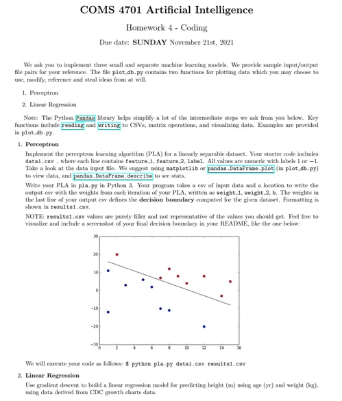
Instructions

Objective

Write a python assignment program to create linear regression and perceptron.

Requirements and Specifications

Source Code

LINEAR REGRESSION import numpy as np import pandas as pd import sys from plot_db import * def gd(x, y, m1, m2, b, learning_rate, iters = 100): """ Implement Gradient Descent Algorithm :param x: x-values. NumPy Array of two columns and N rows :param y: y-values :param m1: slope for variable x1 :param m2: slope for variable x2 :param b: intercept :param learning_rate: learning rate :param iters: Number of iterations :return: optimized values of m and b """ N = len(y) # number of points for i in range(iters): y_new = m1*x[:,0] + m2*x[:,1] +b cost = sum([k**2 for k in (y-y_new)])/N b_gradient = -(2/N)*sum(y-y_new) m1_gradient = -(2/N)*sum(x[:,0]*(y-y_new)) m2_gradient = -(2/N)*sum(x[:,1]*(y-y_new)) # Update values of m and b m1 -= learning_rate*m1_gradient m2 -= learning_rate * m2_gradient b -= learning_rate*b_gradient return m1, m2, b def main(): """ YOUR CODE GOES HERE Implement Linear Regression using Gradient Descent, with varying alpha values and numbers of iterations. Write to an output csv file the outcome betas for each (alpha, iteration #) setting. Please run the file as follows: python3 lr.py data2.csv, results2.csv """ if len(sys.argv) < 3: print("You must provide the input file and the output file as arguments.") sys.exit() input_file = sys.argv[1] output_file = sys.argv[2] # Read input file input_data = pd.read_csv(input_file, header=None).values x = input_data[:, :2] y = input_data[:,2] # Normalize the columns in x such that they have a mean zero x[:,0] = (x[:,0] - np.mean(x[:,0]))/np.std(x[:,0]) x[:, 1] = (x[:, 1] - np.mean(x[:, 1])) / np.std(x[:, 1]) # Use Gradient Descent Algorithm for different learning rates alpha_vals = np.array([0.001, 0.005, 0.01, 0.05, 0.1, 0.5, 1, 5, 10]) fig = plt.figure() ax = fig.add_subplot(111, projection='3d') errors = [] N = len(y) # Create the array to store the values to be written in the output file output_vals = np.zeros((10, 5)) num_iters = 100 for i, alpha in enumerate(alpha_vals): # predict using gradient descent m1, m2, b = gd(x, y, 1, -1, 0, alpha, num_iters) # Compute prediced values y_predict = m1*x[:,0] + m2*x[:,1] + b errors.append(sum([k**2 for k in (y-y_predict)])/N) output_vals[i, :] = np.array([alpha, num_iters, b, m1, m2]) ax.scatter(x[:, 0], x[:, 1], y_predict, marker='o', label=f"alpha = {alpha}") ax.scatter(x[:, 0], x[:, 1], y, c='b', marker='o', label='Data') ax.set_xlabel('X1-axis') ax.set_ylabel('X2-axis') ax.set_zlabel('Y-axis') plt.legend() plt.show() print(errors) """ From the errors printed, the minimum error obtained is 0.0047281... for alpha = 0.5 So now, we will use this alpha and more iterations to obtain a better result """ fig = plt.figure() ax = fig.add_subplot(111, projection='3d') # predict using gradient descent alpha = 0.5 num_iters = 1000 m1, m2, b = gd(x, y, 1, -1, 0, alpha, num_iters) # Compute prediced values y_predict = m1 * x[:, 0] + m2 * x[:, 1] + b error = sum([k**2 for k in (y-y_predict)])/N ax.scatter(x[:, 0], x[:, 1], y_predict, marker='o', label=f"alpha = {alpha}") ax.scatter(x[:, 0], x[:, 1], y, c='b', marker='o', label='Data') ax.set_xlabel('X1-axis') ax.set_ylabel('X2-axis') ax.set_zlabel('Y-axis') plt.legend() plt.show() output_vals[9, :] = np.array([alpha, num_iters, b, m1, m2]) print(f"The error obtained for alpha = {alpha} and 1000 iterations is: {error}") # Finally, write the output file np.savetxt(output_file, output_vals, delimiter=',', fmt='%.4f') if __name__ == "__main__": main() PERCEPTION import pandas as pd import numpy as np import sys import matplotlib.pyplot as plt # Define the function to predict def predict(x, weights, bias): y_ = np.dot(x, weights) + bias return 1.0 if y_ > 0.0 else -1.0 def pla(x, y, learning_rate, epochs = 100, output_file='results1.csv'): # Get number of features and samples n_samples, n_features = x.shape # Initialize weights weights = np.zeros(n_features) # Initialize bias bias = 0.0 # Create array to store the values to be saved into the csv file output_vals = np.zeros((epochs, n_features + 1)) # Now, iterate for i in range(epochs): # Pick each row in the features for j in range(n_samples): xi = x[j, :] # Compute predicted value y_ = predict(xi, weights, bias) # Compute difference dy = (y[j] - y_) # Update weights and bias weights += learning_rate*dy*xi bias += learning_rate*dy output_vals[i,:] = np.array([weights[0], weights[1], bias]) # Print weights and bias # Save csv file np.savetxt(output_file, output_vals, delimiter=',', fmt='%.4f') # Finally, return weights and bias return weights, bias def main(): '''YOUR CODE GOES HERE''' # First, read input file if len(sys.argv) < 3: print("You must provide the input file and the output file as arguments.") sys.exit() input_file = sys.argv[1] output_file = sys.argv[2] # Read input file input_data = pd.read_csv(input_file, header=None, names= ['feature1', 'feature2', 'label']) # Extract x and y values data_np = input_data.values x = data_np[:,:2] y = data_np[:, 2] n_samples, n_features = x.shape # Now compute weights, bias = pla(x, y, 0.1, 100) # Predict y_ = np.zeros((n_samples, 1)) for i in range(n_samples): xi = x[i,:] y_[i] = predict(xi, weights, bias) # Compute accuracy y = y.astype('int') y_ = y_.astype('int') print("The accuracy is: {:.2f}%".format(len(np.where(y==y_.T[0])[0])/n_samples *100.0)) # Plot fig, ax = plt.subplots(nrows = 1, ncols = 2) """ Plot data """ # Pick values with label == -1 x1 = x[np.where(y==-1), 0] x2 = x[np.where(y==-1), 1] ax[0].scatter(x1, x2, c='red', marker='o', label = 'y = -1') # Values with label == 1 x1 = x[np.where(y == 1), 0] x2 = x[np.where(y == 1), 1] ax[0].scatter(x1, x2, c='blue', marker='o', label = 'y = 1') ax[0].set_title('Original Data') """ Plot predicted labels """ # Pick values with label == -1 x1 = x[np.where(y_ == -1), 0] x2 = x[np.where(y_ == -1), 1] ax[1].scatter(x1, x2, c='red', marker='o', label='y = -1') # Values with label == 1 x1 = x[np.where(y_ == 1), 0] x2 = x[np.where(y_ == 1), 1] ax[1].scatter(x1, x2, c='blue', marker='o', label='y = 1') ax[1].set_title('Predicted Data') plt.show() if __name__ == "__main__": """DO NOT MODIFY""" main()