Python Program to Create Data Visualization Assignment Solution

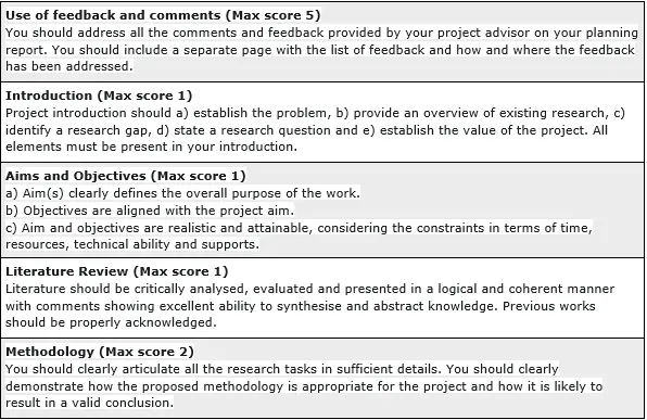
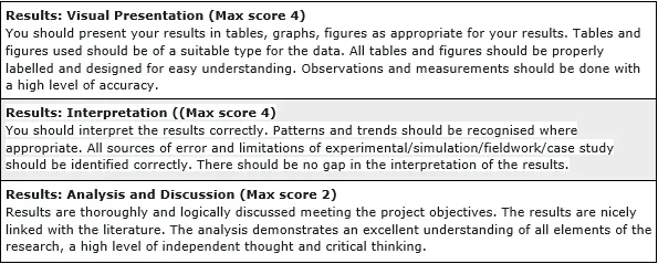
Instructions

Objective

Write a python assignment program to create data visualization.

Requirements and Specifications

Source Code

import pandas as pd import numpy as np import tensorflow as tf import matplotlib.pyplot as plt from datetime import datetime, timedelta # Read data data = pd.read_csv('AEP_hourly.csv') data['Datetime'] = [datetime.strptime(x, '%Y-%m-%d %H:%M:%S') for x in data['Datetime']] data.head() # Visualize Timeseries fig, ax = plt.subplots(figsize=(14,10)) data.plot(x='Datetime', y = 'AEP_MW',ax = ax) plt.grid(True) plt.show() # Let's define a Power Base so we conver the values to P.U $P_{p.u}=\frac{P(MW)}{S_{base}}$ Sbase = data['AEP_MW'].max() data['AEP_MW'] = data['AEP_MW']/Sbase data.head() # Create lag matrices We want a model that can predicts the value of Energy Consumption for a time step $t_{n+1}$ given the values at time-steps $t_{n}, t_{n-1}, t_{n-2},...,t_{n-p}$ where $p$ is thenumber of lags: $y_{t}=f(y(t_{n}),y(t_{n-1}),...,y(t_{n-p}))$ Assume that we have the following values: $Y = [1621.0, 1536.0, 1500.0, 1434.0, 1489.0, 1620.0]$ For $p=3$ the lag values are: $X_{1} = [1621.0, 1536.0, 1500.0]$ First three lags $X_{2} = [1536.0, 1500.0, 1434.0]$ First three lags $X_{3} = [1500.0, 1434.0, 1489.0]$ First three lags Note that, these values will be contained in the same matrix, not in different vectors. So for this case $X$ will be a matrix of size 3x3 y = data['AEP_MW'].tolist() lag = 48 # lag values X = [] Y = [] if len(y) - lag <= 0: X.append(y) else: for i in range(len(y)-lag): Y.append(y[i+lag]) X.append(y[i:(i+lag)]) X, Y = np.array(X), np.array(Y) X = np.reshape(X, (X.shape[0], X.shape[1], 1)) # Split data into Train and Test # Define the size of the train data train_size = 0.7 # 70% n_training = int(len(X)*train_size) X_train = X[:n_training] Y_train = Y[:n_training] X_test = X[n_training:] Y_test = Y[n_training:] print(f"There are {len(X_train)} samples for training and {len(X_test)} for testing") # Model with LSTM (This is only a test model, the real model for this project is in the next cell, so you can skip this cell) model = tf.keras.models.Sequential() model.add(tf.keras.layers.LSTM(50, activation = 'relu', input_shape = (lag, 1))) model.add(tf.keras.layers.Dense(1)) model.compile(optimizer='adam',loss='mse') model.fit(X_train, Y_train, batch_size = 256, epochs = 20, validation_data = (X_test, Y_test)) # Transformer Neural Network (Model with Transformer Encoder) The following cell contains two helper functions def transformer_encoder(inputs, head_size, num_heads, ff_dim, dropout=0): # Normalization x = tf.keras.layers.LayerNormalization(epsilon=1e-6)(inputs) # Attention x = tf.keras.layers.MultiHeadAttention( key_dim=head_size, num_heads=num_heads, dropout=dropout )(x, x) # Dropout layer x = tf.keras.layers.Dropout(dropout)(x) res = x + inputs # Feed Forward Part x = tf.keras.layers.LayerNormalization(epsilon=1e-6)(res) x = tf.keras.layers.Conv1D(filters=ff_dim, kernel_size=1, activation="relu")(x) x = tf.keras.layers.Dropout(dropout)(x) x = tf.keras.layers.Conv1D(filters=inputs.shape[-1], kernel_size=1)(x) return x + res def build_model(input_shape,head_size,num_heads,ff_dim, num_transformer_blocks,mlp_units,dropout=0,mlp_dropout=0): inputs = tf.keras.Input(shape=input_shape) x = inputs # Add encoders for _ in range(num_transformer_blocks): x = transformer_encoder(x, head_size, num_heads, ff_dim, dropout) # Pooling x = tf.keras.layers.GlobalAveragePooling1D(data_format="channels_first")(x) # NN layers for dim in mlp_units: x = tf.keras.layers.Dense(dim, activation="relu")(x) x = tf.keras.layers.Dropout(mlp_dropout)(x) # Output layer outputs = tf.keras.layers.Dense(1)(x) return tf.keras.Model(inputs, outputs) input_shape = X_train.shape[1:] # Shape of data # Create model model = build_model( input_shape, head_size=256, num_heads=4, ff_dim=4, num_transformer_blocks=4, mlp_units=[128], mlp_dropout=0.4, dropout=0.25, ) # Compile model.compile( loss="mse", optimizer='adam', ) # Display summary model.summary() model.fit( X_train, Y_train, validation_data = (X_test, Y_test), epochs=20, batch_size=256 ) # Now, predict for the test dataset and plot Because there are so many samples in the test dataset, the graph will look cluttered. That is why only 500 points will be plotted: ypred = model.predict(X_test) # Constructing the forecast dataframe fc = data.tail(len(ypred)).copy() fc.reset_index(inplace=True) fc['forecast'] = ypred fc = fc.iloc[-500:,:] fig, ax = plt.subplots(figsize=(12,8)) fc.plot(x='Datetime', y='AEP_MW', ax = ax, label = 'Data') fc.plot(x='Datetime', y='forecast', ax = ax, style='r--', label = 'Forecast') plt.legend() plt.grid(True) plt.show() We see that the forecast is not bad but it could be better. It is recommended to increase the number of epochs to reduce the error # Predict N points ahead. Since this dataset is in hours, we will use N = 96 to predict the next 4 days N = 96 y = y[-lag:] X = [] Y = [] if len(y) - lag <= 0: X.append(y) else: for i in range(len(y)-lag): Y.append(y[i+lag]) X.append(y[i:(i+lag)]) X, Y = np.array(X), np.array(Y) X = np.reshape(X, (X.shape[0], X.shape[1], 1)) ypred = [] for _ in range(N): yp = model.predict(X) ypred.append(yp) X = np.append(X, yp) X = np.delete(X, 0) X = np.reshape(X, (1, len(X), 1)) ypred = [y[0][0] for y in ypred] # Constructing the forecast dataframe fc = data.tail(400).copy() fc['type'] = 'original' last_date = max(fc['Datetime']) hat_frame = pd.DataFrame({ 'Datetime': [last_date + timedelta(hours=x + 1) for x in range(N)], 'AEP_MW': ypred }) fig, ax = plt.subplots(figsize=(12,8)) fc.plot(x='Datetime', y = 'AEP_MW', ax = ax, label = 'Data') hat_frame.plot(x='Datetime', y = 'AEP_MW', ax = ax, color='r', label = 'Forecast') plt.legend() plt.grid(True) plt.show()